¶ Introduction
DataSHIELD allows the fitting of generalised linear models (GLM). In Generalised Linear Modelling, the outcome can be modelled as continuous, or categorical (binomial or discrete). The error to use in the model can follow a range of distributions including Gaussian, binomial, gamma and Poisson. In DataSHIELD there are two options for GLMs: (i) virtual pooling, where the results are the same as if you were modelling one dataset, of (ii) study-level meta analysis, whereby models are fit separately in each datasource and results combined. This paper has a detailed explanation of how virtual pooling works with DataSHIELD.
¶ Research question
In this tutorial we will use the Titanic dataset, and attempt to address the question of which characteristics of passengers predicted whether or not they survived. To simulate a situation in which we have data from multiple sources, the dataset has been split into separate parts.
¶ Load libraries
library(dsBaseClient)
library(dsHelper)
library(dsTidyverseClient)
¶ View data
ds.colnames("titanic")
## $server1
##  [1] "entity_id" "Survived"  "Pclass"    "Name"      "Sex"
##  [6] "Age"       "SibSp"     "Parch"     "Ticket"    "Fare"
## [11] "Cabin"     "Embarked"
##
## $server2
##  [1] "Survived" "Pclass"   "Name"     "Sex"      "Age"      "SibSp"
##  [7] "Parch"    "Ticket"   "Fare"     "Cabin"    "Embarked"
¶ Fit 1-stage model with binomial link function
Let's use a simple model where probability of survival is predicted by sex, age and ticket fare. First, lets create a variable for study so that we can include this as a covariate.
ds.mutate(
  df.name = "titanic",
  tidy_expr = list(cohort = 0),
  newobj = "titanic",
  datasources = conns["server1"]
)

ds.mutate(
  df.name = "titanic",
  tidy_expr = list(cohort = 1),
  newobj = "titanic",
  datasources = conns["server2"]
)
Now lets fit a simple logistic regression model. The model is passed as a character string to formula, the server-side data source is passed as a character string to data, and the link function is specified under family. As we are fitting a logistic regression model we chose binary, if we had a continuous outcome we could chose gaussian instead.
model_1 <- ds.glm(
  formula = "Survived ~ Sex + Age + Fare + cohort",
  data = "titanic",
  family = "binomial"
)
We can see the model output here:
model_1
## $Nvalid
## [1] 714
##
## $Nmissing
## [1] 177
##
## $Ntotal
## [1] 891
##
## $disclosure.risk
##         RISK OF DISCLOSURE
## server1                  0
## server2                  0
##
## $errorMessage
##         ERROR MESSAGES
## server1 "No errors"
## server2 "No errors"
##
## $nsubs
## [1] 714
##
## $iter
## [1] 6
##
## $family
##
## Family: binomial
## Link function: logit
##
##
## $formula
## [1] "Survived ~ Sex + Age + Fare + cohort"
##
## $coefficients
##                Estimate  Std. Error    z-value      p-value low0.95CI.LP
## (Intercept)  0.80848433 0.249827417   3.236171 1.211446e-03   0.31883159
## Sexmale     -2.37096211 0.191603626 -12.374307 3.599877e-35  -2.74649831
## Age         -0.01145066 0.006541126  -1.750564 8.002102e-02  -0.02427103
## Fare         0.01292142 0.002685862   4.810904 1.502494e-06   0.00765723
## cohort       0.32236993 0.188196257   1.712946 8.672256e-02  -0.04648795
##             high0.95CI.LP       P_OR low0.95CI.P_OR high0.95CI.P_OR
## (Intercept)   1.298137067 0.69178643     0.57903947       0.7855213
## Sexmale      -1.995425900 0.09339083     0.06415211       0.1359557
## Age           0.001369711 0.98861465     0.97602114       1.0013706
## Fare          0.018185614 1.01300526     1.00768662       1.0183520
## cohort        0.691227820 1.38039534     0.95457606       1.9961650
##
## $dev
## [1] 713.1114
##
## $df
## [1] 709
##
## $output.information
## [1] "SEE TOP OF OUTPUT FOR INFORMATION ON MISSING DATA AND ERROR MESSAGES"
Alternatively, we can use a helper function from the dsHelper package to return the model output in a more readable form:
dh.lmTab(
  model = model_1,
  type = "glm_ipd",
  family = "binomial",
  direction = "wide",
  ci_format = "separate",
  exponentiate = FALSE)
## # A tibble: 5 × 7
##   variable    est    se pvalue lowci uppci n_obs
##   <chr>     <dbl> <dbl>  <dbl> <dbl> <dbl> <int>
## 1 intercept  0.81  0.25   0     0.32  1.3    714
## 2 Sexmale   -2.37  0.19   0    -2.75 -2      714
## 3 Age       -0.01  0.01   0.08 -0.02  0      714
## 4 Fare       0.01  0      0     0.01  0.02   714
## 5 cohort     0.32  0.19   0.09 -0.05  0.69   714
¶ 2-Stage logistic regression model
The other main type of functionality in DataSHIELD are two-stage models. Let's fit exactly the same model as before, but using a 2-stage approach:]
model_2 <- ds.glmSLMA(
  formula = "Survived ~ Sex + Age + Fare + cohort",
  dataName = "titanic",
  family = "binomial"
)
Again, we can retrieve the neat output:
model_2_tab <- dh.lmTab(
  model = model_2,
  type = "glm_slma",
  family = "binomial",
  direction = "wide",
  ci_format = "separate",
  coh_names = c("cohort1", "cohort2"),
  exponentiate = TRUE)

model_2_tab
## # A tibble: 12 × 9
##    cohort   variable    est    se pvalue n_obs n_coh lowci uppci
##    <chr>    <chr>     <dbl> <dbl>  <dbl> <dbl> <dbl> <dbl> <dbl>
##  1 cohort1  intercept  3.24  0.34   0      357     1  1.66  6.34
##  2 cohort1  Sexmale    0.08  0.27   0      357     1  0.05  0.13
##  3 cohort1  Age        0.99  0.01   0.13   357     1  0.97  1
##  4 cohort1  Fare       1.01  0      0.01   357     1  1     1.01
##  5 cohort2  intercept  1.86  0.34   0.07   357     1  0.95  3.64
##  6 cohort2  Sexmale    0.12  0.28   0      357     1  0.07  0.2
##  7 cohort2  Age        0.99  0.01   0.17   357     1  0.97  1.01
##  8 cohort2  Fare       1.03  0.01   0      357     1  1.02  1.04
##  9 combined intercept  2.46  0.24  NA      714     2  1.53  3.95
## 10 combined Sexmale    0.1   0.19  NA      714     2  0.07  0.14
## 11 combined Age        0.99  0.01  NA      714     2  0.97  1
## 12 combined Fare       1.02  0.01  NA      714     2  1     1.03
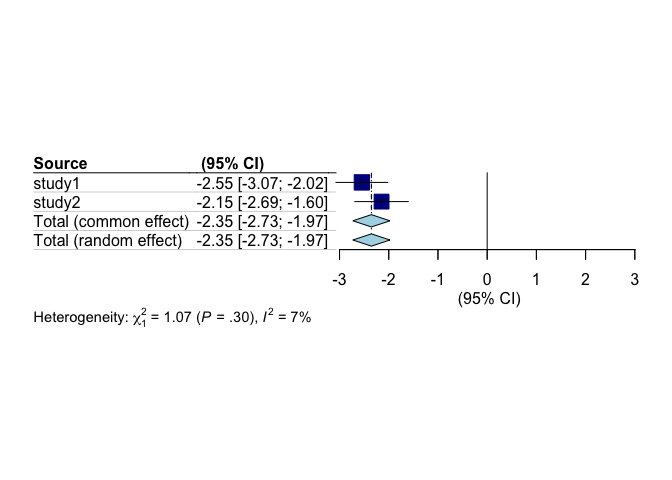
We can also plot the output in a forest plot:
ds.forestplot(model_2)
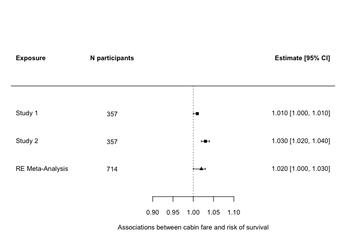
As we saw in the tutorial on plotting, we can make our own custom plots using the summary statistics we have returned. The metafor package contains the function forest which can be used to make neat plots. The downside is that lining things up is a faff, and involves a fair bit of trial an error. Assume that our exposure of interest is fare paid, we can make the following forest plot:
library(metafor)

plot_data <- model_2_tab |>
  dplyr::filter(variable == "Fare")

forest(
  x = plot_data$est,
  ci.lb = plot_data$lowci,
  ci.ub = plot_data$uppci,
  ilab = plot_data$n_obs,
  ilab.xpos = 0.8,
  slab = c("Study 1", "Study 2", "RE Meta-Analysis"),
  annotate = T,
  xlab = "Associations between cabin fare and risk of survival",
  cex = 0.8,
  cex.axis = 0.8,
  header = c("Exposure", "Estimate [95% CI]"),
  refline = 1,
  xlim = c(0.55, 1.35),
  alim = c(0.9, 1.1),
  steps = 5,
  digits = c(3, 2),
  pch = c(15, 15, 17),
  psize = 1)

text(0.8, 5, "N participants", cex = 0.8, font = 2)
¶ Logout
datashield.logout(conns)