¶ Introduction
Other tutorials in this section show how to perform individual operations in DataSHIELD. This tutorial takes a specific research question and shows how to perform an entire analysis, from start to finish. As preqrequisite, please read the tutorials '1. Key concepts' and '2. Logging in to demo servers'.
¶ Research question
The question we will address in this tutorial is: > Among Titanic passengers, was travelling alone associated with a lower chance of survival, after accounting for age, sex, ticket class and port of embarkation? We will use passenger data from the Titanic disaster. On the demo servers this is split across two servers, letting us imagine two data custodians ("cohorts") who each hold the records for different passengers and cannot share individual-level data.
Survived ~ is_alone + age_cat + Sex + Pclass + Embarked
¶ Loading packages
First, we load the packages that we need for the analysis.
library(DSI)
library(DSMolgenisArmadillo)
library(DSOpal)
library(dsBaseClient)
library(dsTidyverseClient)
library(dsHelper)
¶ Logging in and loading data
Next, we log into to the two demo servers which hold the data.
armadillo_url <- "https://armadillo-playground.molgenis.net/"
credentials <- armadillo.get_credentials(server = armadillo_url)
## [1] "We're opening a browser so you can log in with code FANN-XXWA"
builder <- DSI::newDSLoginBuilder()
builder$append(
  server = "server1",
  url = armadillo_url,
  token = credentials@access_token,
  driver = "ArmadilloDriver",
  profile = "molgenis-base"
)
builder$append(
  server = "server2",
  url = "https://opal-demo.obiba.org/",
  user = "dsuser",
  password = "P@ssw0rd",
  driver = "OpalDriver",
  profile = "default"
)

logindata <- builder$build()
conns <- datashield.login(
  logins = logindata,
  assign = FALSE
)
Next, we 'assign' the data. This mean to copy the data from the data store into our remote session. Note this does not mean that we can see the data, just that it is available in this session for analysis with DataSHIELD.
datashield.assign.table(
  conns = conns["server1"],
  symbol = "titanic",
  table = "example-datasets/data/titanic_1"
)
datashield.assign.table(
  conns = conns["server2"],
  symbol = "titanic",
  table = "TITANIC_NEWCOMERS_WORKSHOP.titanic_server_2"
)
We can see what has been created by checking what is available in the remote workspace:
ds.ls()
## $server1
## $server1$environment.searched
## [1] "R_GlobalEnv"
##
## $server1$objects.found
## [1] "titanic"
##
##
## $server2
## $server2$environment.searched
## [1] "R_GlobalEnv"
##
## $server2$objects.found
## [1] "titanic"
There is one object in each cohort, "titanic". Now we can inspect other properties of that dataset, like the dimensions and column names.
ds.dim("titanic")
## $`dimensions of titanic in server1`
## [1] 444  12
##
## $`dimensions of titanic in server2`
## [1] 447  11
##
## $`dimensions of titanic in combined studies`
## [1] 891  12
ds.colnames("titanic")
## $server1
##  [1] "entity_id" "Survived"  "Pclass"    "Name"      "Sex"       "Age"
##  [7] "SibSp"     "Parch"     "Ticket"    "Fare"      "Cabin"     "Embarked"
##
## $server2
##  [1] "Survived" "Pclass"   "Name"     "Sex"      "Age"      "SibSp"
##  [7] "Parch"    "Ticket"   "Fare"     "Cabin"    "Embarked"
Now let's start working with the data.
¶ 1. Checking what is available
In an ideal situation you will be working with perfectly harmonised data - all data sources will have the same variable of the same type. However, in real life situations things are not so neat. The first thing to check therefore is which variables are available and whether they are of the same class (DataSHIELD generally expects these two criteria to be met).
analysis_vars <- c("Survived", "Pclass", "Name", "Sex", "Age", "SibSp", "Parch", "Ticket", "Fare", "Cabin", "Embarked")

classes <- dh.classDiscrepancy(
  df = "titanic",
  vars = analysis_vars,
  conns = conns)

classes
## # A tibble: 11 × 4
##    variable discrepancy server1   server2
##    <chr>    <chr>       <chr>     <chr>
##  1 Survived yes         numeric   factor
##  2 Pclass   yes         numeric   factor
##  3 Name     no          character character
##  4 Sex      no          character character
##  5 Age      no          numeric   numeric
##  6 SibSp    no          numeric   numeric
##  7 Parch    no          numeric   numeric
##  8 Ticket   no          character character
##  9 Fare     no          numeric   numeric
## 10 Cabin    no          character character
## 11 Embarked yes         character factor
We can see there is a problem with "Survived", "Pclass", "Embarked" and "Sex". These should be a factor in all studies. We can set them as follows:
ds.asFactor("titanic$Survived", newobj = "Survived") ## Convert to factor
## $all.unique.levels
## [1] "0" "1"
##
## $return.message
## [1] "Data object <Survived> correctly created in all specified data sources"
ds.asFactor("titanic$Pclass", newobj = "Pclass")
## $all.unique.levels
## [1] "1" "2" "3"
##
## $return.message
## [1] "Data object <Pclass> correctly created in all specified data sources"
ds.asFactor("titanic$Embarked", newobj = "Embarked")
## $all.unique.levels
## [1] "C" "Q" "S"
##
## $return.message
## [1] "Data object <Embarked> correctly created in all specified data sources"
ds.asFactor("titanic$Sex", newobj = "Sex")
## $all.unique.levels
## [1] "female" "male"
##
## $return.message
## [1] "Data object <Sex> correctly created in all specified data sources"
ds.select(
  df.name = "titanic",
  tidy_expr = list(-Survived, -Pclass, -Embarked, -Sex),
  newobj = "titanic") ## Remove original variables

ds.dataFrame(
  x = c("titanic", "Survived", "Pclass", "Embarked", "Sex"),
  newobj = "titanic") ## Join columns back into original data frame
## $is.object.created
## [1] "A data object <titanic> has been created in all specified data sources"
##
## $validity.check
## [1] "<titanic> appears valid in all sources"
Note, ds.mutate is available for many datashield operations. However, because factor conversion carries disclosure risk and requires complex checks, it is not permitted to be used via ds.mutate and thus we have to handle factors via ds.assign and ds.dataFrame.
We can check that has worked:
ds.colnames("titanic")
## $server1
##  [1] "entity_id" "Name"      "Age"       "SibSp"     "Parch"     "Ticket"
##  [7] "Fare"      "Cabin"     "Survived"  "Pclass"    "Embarked"  "Sex"
##
## $server2
##  [1] "Name"     "Age"      "SibSp"    "Parch"    "Ticket"   "Fare"
##  [7] "Cabin"    "Survived" "Pclass"   "Embarked" "Sex"
classes_fixed <- dh.classDiscrepancy(
  df = "titanic",
  vars = analysis_vars,
  conns = conns)

classes_fixed
## # A tibble: 11 × 4
##    variable discrepancy server1   server2
##    <chr>    <chr>       <chr>     <chr>
##  1 Survived no          factor    factor
##  2 Pclass   no          factor    factor
##  3 Name     no          character character
##  4 Sex      no          factor    factor
##  5 Age      no          numeric   numeric
##  6 SibSp    no          numeric   numeric
##  7 Parch    no          numeric   numeric
##  8 Ticket   no          character character
##  9 Fare     no          numeric   numeric
## 10 Cabin    no          character character
## 11 Embarked no          factor    factor
¶ 2. Deriving new variables
Whilst you will normally be working with harmonised data, often additional data preparation is required. This can included transforming continuous variables to categorical variables, collapsing the categories of categorical variables, or applying other transformations (e.g. square root or z-scores).
¶ Deriving a categorical variable from a continuous one
Here we bin the continuous Age into age groups with case_when, then convert the result to a factor.
ds.mutate(
  df.name = "titanic",
  tidy_expr = list(
    age_cat = case_when(
      Age < 16 ~ 1,
      Age >= 16 & Age < 60 ~ 2,
      Age >= 60 ~ 3
      )
    ),
  newobj = "titanic"
)
¶ Deriving a variable using arithmetic
We want to derive a variable indicating the overall family size. SibSp is the number of siblings or spouses aboard and Parch the number of parents or children aboard, so SibSp + Parch + 1 (adding the passenger themselves) gives the total family_size.
ds.mutate(
  df.name = "titanic",
  tidy_expr = list(
    family_size = SibSp + Parch + 1
  ),
  newobj = "titanic"
)
¶ Deriving an indicator variable
A passenger is travelling alone when their family size is one; if_else returns 1 if so and 0 otherwise.
ds.mutate(
  df.name = "titanic",
  tidy_expr = list(
    is_alone = if_else(family_size == 1, 1, 0)
  ),
  newobj = "titanic"
)
¶ Converting these to factor
These indicator variables need to be factor, not numeric. Let's convert them like before:
ds.asFactor("titanic$age_cat", "age_cat")
## $all.unique.levels
## [1] "1" "2" "3"
##
## $return.message
## [1] "Data object <age_cat> correctly created in all specified data sources"
ds.asFactor("titanic$family_size", "family_size")
## $all.unique.levels
## [1] "1"  "2"  "3"  "4"  "5"  "6"  "7"  "8"  "11"
##
## $return.message
## [1] "Data object <family_size> correctly created in all specified data sources"
ds.asFactor("titanic$is_alone", "is_alone")
## $all.unique.levels
## [1] "0" "1"
##
## $return.message
## [1] "Data object <is_alone> correctly created in all specified data sources"
ds.select("titanic", list(-age_cat, -family_size, -is_alone), newobj = "titanic")
ds.dataFrame(c("titanic", "age_cat", "family_size", "is_alone"), newobj = "titanic")
## $is.object.created
## [1] "A data object <titanic> has been created in all specified data sources"
##
## $validity.check
## [1] "<titanic> appears valid in all sources"
¶ Dropping variables
We can drop the old variables that we no longer need for the analysis:
ds.colnames("titanic")
## $server1
##  [1] "entity_id"   "Name"        "Age"         "SibSp"       "Parch"
##  [6] "Ticket"      "Fare"        "Cabin"       "Survived"    "Pclass"
## [11] "Embarked"    "Sex"         "age_cat"     "family_size" "is_alone"
##
## $server2
##  [1] "Name"        "Age"         "SibSp"       "Parch"       "Ticket"
##  [6] "Fare"        "Cabin"       "Survived"    "Pclass"      "Embarked"
## [11] "Sex"         "age_cat"     "family_size" "is_alone"
ds.select(
  df.name = "titanic",
  tidy_expr = list(-Age, -SibSp, -Parch),
  newobj = "titanic")

ds.colnames("titanic")
## $server1
##  [1] "entity_id"   "Name"        "Ticket"      "Fare"        "Cabin"
##  [6] "Survived"    "Pclass"      "Embarked"    "Sex"         "age_cat"
## [11] "family_size" "is_alone"
##
## $server2
##  [1] "Name"        "Ticket"      "Fare"        "Cabin"       "Survived"
##  [6] "Pclass"      "Embarked"    "Sex"         "age_cat"     "family_size"
## [11] "is_alone"
¶ 3. Defining the analysis sample
We keep only passengers eligible for the analysis: those with the outcome recorded, and fare-paying passengers (a Fare of 0 flags crew and complimentary tickets).
ds.filter(
  df.name = "titanic",
  tidy_expr = list(!is.na(Survived) & Fare > 0),
  newobj = "analysis_df"
)
Check the dimensions to see that we now have fewer rows:
ds.dim(x = "titanic")
## $`dimensions of titanic in server1`
## [1] 444  12
##
## $`dimensions of titanic in server2`
## [1] 447  11
##
## $`dimensions of titanic in combined studies`
## [1] 891  12
ds.dim(x = "analysis_df")
## $`dimensions of analysis_df in server1`
## [1] 438  12
##
## $`dimensions of analysis_df in server2`
## [1] 438  11
##
## $`dimensions of analysis_df in combined studies`
## [1] 876  12
¶ 4. Describing the sample: a "Table 1"
Most analyses begin with a table describing the sample. We use dh.getStats to summarise our variables across both cohorts.
stats <- dh.getStats(
  df = "titanic",
  vars = c("Survived", "is_alone", "age_cat", "Sex", "Pclass", "Embarked")
)
The result splits into categorical and continuous summaries:
stats$categorical
## # A tibble: 63 × 10
##    variable cohort   category value cohort_n valid_n missing_n perc_valid
##    <chr>    <chr>    <fct>    <int>    <int>   <int>     <int>      <dbl>
##  1 Embarked combined C          168      891     889         2      18.9
##  2 Embarked combined Q           77      891     889         2       8.66
##  3 Embarked combined S          644      891     889         2      72.4
##  4 Embarked combined <NA>         2      891      NA        NA      NA
##  5 Pclass   combined 1          216      891     891         0      24.2
##  6 Pclass   combined 2          184      891     891         0      20.6
##  7 Pclass   combined 3          491      891     891         0      55.1
##  8 Pclass   combined <NA>         0      891      NA        NA      NA
##  9 Sex      combined female     314      891     891         0      35.2
## 10 Sex      combined male       577      891     891         0      64.8
## # ℹ 53 more rows
## # ℹ 2 more variables: perc_missing <dbl>, perc_total <dbl>
stats$continuous
## # A tibble: 0 × 15
## # ℹ 15 variables: variable <chr>, cohort <chr>, mean <dbl>, std.dev <dbl>,
## #   perc_5 <dbl>, perc_10 <dbl>, perc_25 <dbl>, perc_50 <dbl>, perc_75 <dbl>,
## #   perc_90 <dbl>, perc_95 <dbl>, valid_n <dbl>, cohort_n <int>,
## #   missing_n <dbl>, missing_perc <dbl>
The summary numbers have already been returned from the servers, so we can format them locally into a publication-ready table with dh.createTableOne. First we supply human-readable labels for the variables and their categories:
library(dplyr)

var_labels <- tibble(
  variable = c("Survived", "is_alone", "age_cat", "Sex", "Pclass", "Embarked"),
  var_label = c(
    "Survived", "Travelling alone", "Age category", "Sex",
    "Passenger class", "Port of embarkation")
)

cat_labels <- tibble(
  variable = c(
    "Survived", "Survived",
    "is_alone", "is_alone",
    "age_cat", "age_cat", "age_cat",
    "Sex", "Sex",
    "Pclass", "Pclass", "Pclass",
    "Embarked", "Embarked", "Embarked"
  ),
  category = c(
    "0", "1",
    "0", "1",
    "1", "2", "3",
    "female", "male",
    "1", "2", "3",
    "C", "Q", "S"
  ),
  cat_label = c(
    "Died", "Survived",
    "Not alone", "Travelling alone",
    "Child (<16)", "Adult (16-59)", "Elderly (60+)",
    "Female", "Male",
    "1st class", "2nd class", "3rd class",
    "Cherbourg", "Queenstown", "Southampton"
  )
)
Then we pass the summary statistics and labels to dh.createTableOne. This returns a formatted table which can be saved as a .csv and used in your article.
table_one <- dh.createTableOne(
  stats = stats,
  vars = var_labels$variable,
  var_labs = var_labels,
  cat_labs = cat_labels,
  type = "both",
  cont_format = "med_iqr",
  inc_missing = TRUE,
  perc_denom = "valid"
)

table_one
## # A tibble: 21 × 5
##    variable         category         combined   server1    server2
##    <chr>            <chr>            <chr>      <chr>      <chr>
##  1 Survived         Survived         342 (38.4) 173 (39)   169 (37.8)
##  2 Survived         Died             549 (61.6) 271 (61)   278 (62.2)
##  3 Survived         <NA>             0 (0)      0 (0)      0 (0)
##  4 Travelling alone Travelling alone 537 (60.3) 254 (57.2) 283 (63.3)
##  5 Travelling alone Not alone        354 (39.7) 190 (42.8) 164 (36.7)
##  6 Travelling alone <NA>             0 (0)      0 (0)      0 (0)
##  7 Age category     Child (<16)      83 (11.6)  42 (11.8)  41 (11.5)
##  8 Age category     Adult (16-59)    605 (84.7) 304 (85.2) 301 (84.3)
##  9 Age category     Elderly (60+)    26 (3.64)  11 (3.08)  15 (4.2)
## 10 Age category     <NA>             177 (19.9) 87 (19.6)  90 (20.1)
## # ℹ 11 more rows
¶ 5. Fitting the model
With the data prepared and the sample defined, we can fit the model. First we add a cohort indicator so the pooled estimate can account for differences between the two archives.
ds.mutate(
  df.name = "analysis_df",
  tidy_expr = list(cohort = 0),
  newobj = "analysis_df",
  datasources = conns["server1"]
)

ds.mutate(
  df.name = "analysis_df",
  tidy_expr = list(cohort = 1),
  newobj = "analysis_df",
  datasources = conns["server2"]
)
¶ One-stage (virtual pooling)
The one-stage approach pools the individual-level data virtually, as if it were one dataset. We can see that travelling along is associated with an OR of 1.33 of death (CI 0.86 - 2.06), adjusting for hypothesised confounding factors.
model_ipd <- ds.glm(
  formula = "Survived ~ is_alone + age_cat + Sex + Pclass + Embarked + cohort",
  data = "analysis_df",
  family = "binomial"
)

dh.lmTab(
  model = model_ipd,
  type = "glm_ipd",
  family = "binomial",
  direction = "wide",
  ci_format = "separate",
  exponentiate = TRUE
)
## # A tibble: 10 × 7
##    variable    est    se pvalue lowci  uppci n_obs
##    <chr>     <dbl> <dbl>  <dbl> <dbl>  <dbl> <int>
##  1 intercept 47.5   0.44   0    19.9  113.     705
##  2 is_alone1  1.33  0.22   0.2   0.86   2.06   705
##  3 age_cat2   0.25  0.33   0     0.13   0.49   705
##  4 age_cat3   0.1   0.64   0     0.03   0.34   705
##  5 Sexmale    0.08  0.22   0     0.05   0.12   705
##  6 Pclass2    0.36  0.28   0     0.21   0.63   705
##  7 Pclass3    0.11  0.27   0     0.06   0.18   705
##  8 EmbarkedQ  0.45  0.56   0.16  0.15   1.36   705
##  9 EmbarkedS  0.62  0.27   0.08  0.37   1.06   705
## 10 cohort     1.23  0.2    0.3   0.83   1.82   705
¶ Two-stage (study-level meta-analysis)
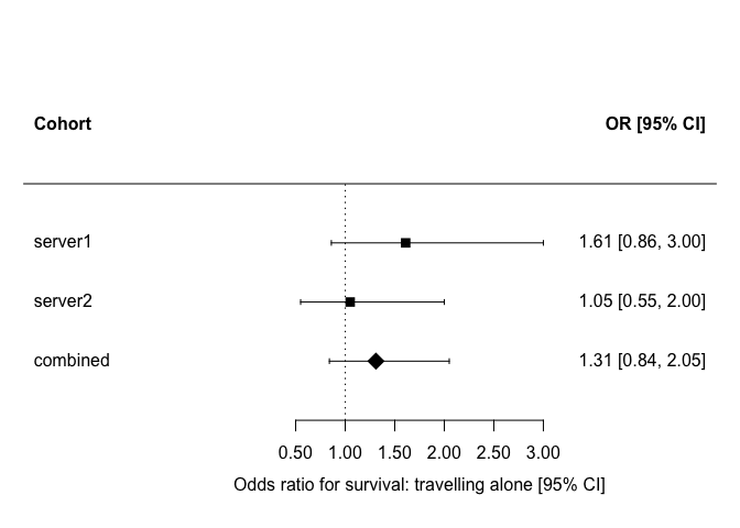
The two-stage approach fits the model separately in each cohort, then meta-analyses the estimates. This approach is useful when you want to specifically model the heterogeneity between data sources. Using this approach the estimated OR of travelling alone is higher (1.31), but confidence intervals still cross 1 (CI 0.84-2.05)
model_slma <- ds.glmSLMA(
  formula = "Survived ~ is_alone + age_cat + Sex + Pclass + Embarked",
  dataName = "analysis_df",
  family = "binomial"
)

dh.lmTab(
  model = model_slma,
  type = "glm_slma",
  family = "binomial",
  direction = "wide",
  ci_format = "separate",
  coh_names = c("server1", "server2"),
  exponentiate = TRUE
) %>% print(n = Inf)
## # A tibble: 27 × 9
##    cohort   variable     est    se pvalue n_obs n_coh lowci  uppci
##    <chr>    <chr>      <dbl> <dbl>  <dbl> <dbl> <dbl> <dbl>  <dbl>
##  1 server1  intercept  18.6   0.59   0      352     1  5.85  59.2
##  2 server1  is_alone1   1.61  0.32   0.14   352     1  0.86   3
##  3 server1  age_cat2    0.33  0.46   0.02   352     1  0.13   0.83
##  4 server1  age_cat3    0.08  1.06   0.02   352     1  0.01   0.65
##  5 server1  Sexmale     0.07  0.3    0      352     1  0.04   0.12
##  6 server1  Pclass2     0.45  0.42   0.06   352     1  0.2    1.03
##  7 server1  Pclass3     0.15  0.4    0      352     1  0.07   0.34
##  8 server1  EmbarkedQ   1.56  0.77   0.56   352     1  0.35   7.02
##  9 server1  EmbarkedS   1.05  0.4    0.91   352     1  0.48   2.31
## 10 server2  intercept 134.    0.65   0      353     1 37.4  478.
## 11 server2  is_alone1   1.05  0.33   0.87   353     1  0.55   2
## 12 server2  age_cat2    0.21  0.5    0      353     1  0.08   0.55
## 13 server2  age_cat3    0.1   0.83   0.01   353     1  0.02   0.52
## 14 server2  Sexmale     0.08  0.33   0      353     1  0.04   0.16
## 15 server2  Pclass2     0.29  0.4    0      353     1  0.13   0.64
## 16 server2  Pclass3     0.07  0.39   0      353     1  0.03   0.16
## 17 server2  EmbarkedQ   0.09  1.16   0.04   353     1  0.01   0.85
## 18 server2  EmbarkedS   0.39  0.39   0.02   353     1  0.18   0.84
## 19 combined intercept  48.1   0.7   NA      705     2 12.3  188.
## 20 combined is_alone1   1.31  0.23  NA      705     2  0.84   2.05
## 21 combined age_cat2    0.27  0.34  NA      705     2  0.14   0.52
## 22 combined age_cat3    0.09  0.65  NA      705     2  0.03   0.34
## 23 combined Sexmale     0.07  0.22  NA      705     2  0.05   0.11
## 24 combined Pclass2     0.36  0.29  NA      705     2  0.2    0.63
## 25 combined Pclass3     0.11  0.28  NA      705     2  0.06   0.18
## 26 combined EmbarkedQ   0.49  0.98  NA      705     2  0.07   3.33
## 27 combined EmbarkedS   0.63  0.35  NA      705     2  0.32   1.25
¶ Visualising the two-stage results
A forest plot shows each cohort's estimate alongside the pooled one (there is no equivalent for the one-stage model, which returns a single pooled estimate). We pass the tidy dh.lmTab output to metafor::forest, here for the exposure is_alone.
library(metafor)

slma_table <- dh.lmTab(
  model = model_slma,
  type = "glm_slma",
  family = "binomial",
  direction = "wide",
  ci_format = "separate",
  coh_names = c("server1", "server2"),
  exponentiate = TRUE
)

exposure_forest <- slma_table |>
  dplyr::filter(startsWith(variable, "is_alone"))

is_combined <- exposure_forest$cohort == "combined"

forest(
  x     = exposure_forest$est,
  ci.lb = exposure_forest$lowci,
  ci.ub = exposure_forest$uppci,
  slab  = exposure_forest$cohort,
  xlab    = "Odds ratio for survival: travelling alone [95% CI]",
  header  = c("Cohort", "OR [95% CI]"),
  refline = 1,
  col     = "black",
  pch     = ifelse(is_combined, 18, 15),
  psize   = ifelse(is_combined, 2.2, 1.2),
  digits  = c(2, 2)
)
¶ 6. Supplementary analysis: multiple imputation
The main analysis above uses only passengers with complete data. This risks loses power and may make results more susceptable to selection bias. As a supplementary analysis, we can instead use multiple imputation to make use of the partially-complete records and then repeat the analysis. This has three steps: create the imputed datasets, fit the model on each of them, pool the results, and then combine the pulled results by 2-stage meta-analysis across data sources.
¶ Creating the imputed datasets
We impute the confounders, predicting each from all the other analysis variables. First we build a data frame holding just the variables for the imputation model:
ds.select(
  df.name = "analysis_df",
  tidy_expr = list(Survived, is_alone, age_cat, Sex, Pclass, Embarked, Fare),
  newobj = "imp_df"
)
This keeps the outcome, the exposure, the four confounders and Fare as an auxiliary. We leave out the identifiers Name, Ticket and Cabin (no information for imputation) and family_size (collinear with is_alone, which is derived from it).
We start with a dry run (maxit = 0): no imputation is done, but ds.mice returns the method and predictorMatrix it picks automatically from each column's type.
dry_run <- ds.mice(data = "imp_df", maxit = 0)
mice picks the method from each column's type: pmm for numeric, logreg for binary factors and polyreg for multi-category factors. It then blanks out ("") any column with no missing values, since there is nothing there to impute.
dry_run$server1$method
##  Survived  is_alone   age_cat       Sex    Pclass  Embarked      Fare
##        ""        "" "polyreg"        ""        "" "polyreg"        ""
Only age_cat and Embarked have missing values, so they are the only columns that will be imputed; everything else is complete and acts purely as a predictor. The automatic choice is what we want here, so we pass it through unchanged.
Now the imputation itself. With no predictorMatrix supplied, each imputed column is predicted by all the others; seed = "fixed" makes it reproducible.
imputation <- ds.mice(
  data = "imp_df",
  seed = "fixed",
  newobj_mids = "mids_object",
  newobj_df = "imputationSet"
)
This creates the imputed data on each server: the pooled mids_object, and m = 5 completed data frames named imputationSet.1 to imputationSet.5:
ds.ls()
## $server1
## $server1$environment.searched
## [1] "R_GlobalEnv"
##
## $server1$objects.found
##  [1] "age_cat"         "analysis_df"     "Embarked"        "family_size"
##  [5] "imp_df"          "imputationSet.1" "imputationSet.2" "imputationSet.3"
##  [9] "imputationSet.4" "imputationSet.5" "is_alone"        "mids_object"
## [13] "new.glm.obj"     "Pclass"          "Sex"             "Survived"
## [17] "titanic"
##
##
## $server2
## $server2$environment.searched
## [1] "R_GlobalEnv"
##
## $server2$objects.found
##  [1] "age_cat"         "analysis_df"     "Embarked"        "family_size"
##  [5] "imp_df"          "imputationSet.1" "imputationSet.2" "imputationSet.3"
##  [9] "imputationSet.4" "imputationSet.5" "is_alone"        "mids_object"
## [13] "new.glm.obj"     "Pclass"          "Sex"             "Survived"
## [17] "titanic"
¶ Fitting the model on the imputed datasets
We perform the analysis in 3 stages: 1. Fit the model separately, for each cohort on each imputed dataset. 2. Within cohort, combine the estimates across the 5 datasets using Rubin's rules. 3. Meta-analyse the pooled estimates across cohorts.
For each coefficient, dh.pool takes the m estimates and standard errors --- one per imputed dataset --- and combines them:
pooled_mean = mean(est)
within      = mean(se^2)
between     = sum((est - pooled_mean)^2) / (m - 1)
pooled_se   = sqrt(within + between + between / m)
CI          = pooled_mean +/- qnorm(0.975) * pooled_se
Step 1: fit each cohort separately. ds.glmSLMA fits the model separately in every cohort in a single call, so we do not need to loop over the servers ourselves. It also meta-analyses the results for us, but we ignore that here --- we want to pool across imputations before combining the cohorts, not after:
library(purrr)
imputed_sets <- paste0("imputationSet.", 1:5)

imputed_slma <- imputed_sets |>
  map(~ ds.glmSLMA(
    formula = "Survived ~ is_alone + age_cat + Sex + Pclass + Embarked",
    dataName = .x,
    family = "binomial"
  ))
Step 2: pool across imputations, within each cohort. dh.pool drops the combined row that ds.glmSLMA added and applies the same Rubin's rules as before, once per cohort. Note exponentiate = FALSE: the meta-analysis in step 3 needs the estimates and their standard errors on the same scale, so we stay on the log-odds scale and exponentiate only at the very end.
pooled_by_cohort <- dh.pool(
  imputed_glm = imputed_slma,
  type = "glm_slma",
  family = "binomial",
  coh_names = c("server1", "server2"),
  exponentiate = FALSE
)

pooled_by_cohort
## # A tibble: 18 × 11
##    variable  cohort n_obs pooled_mean within_var between_var pooled_se z_value
##    <chr>     <chr>  <dbl>       <dbl>      <dbl>       <dbl>     <dbl>   <dbl>
##  1 EmbarkedQ serve…   438      0.827      0.292     0.00402      0.545   1.52
##  2 EmbarkedS serve…   438     -0.0989     0.124     0.000166     0.352  -0.281
##  3 Pclass2   serve…   438     -0.722      0.155     0.00574      0.402  -1.80
##  4 Pclass3   serve…   438     -1.93       0.130     0.00483      0.368  -5.25
##  5 Sexmale   serve…   438     -2.80       0.0758    0.00164      0.279 -10.0
##  6 age_cat2  serve…   438     -1.17       0.172     0.0222       0.446  -2.62
##  7 age_cat3  serve…   438     -2.84       0.819     0.186        1.02   -2.78
##  8 intercept serve…   438      3.13       0.286     0.0146       0.551   5.68
##  9 is_alone1 serve…   438      0.485      0.0859    0.00176      0.297   1.63
## 10 EmbarkedQ serve…   438     -1.07       0.367     0.0172       0.622  -1.72
## 11 EmbarkedS serve…   438     -0.794      0.112     0.000937     0.336  -2.36
## 12 Pclass2   serve…   438     -1.07       0.138     0.00213      0.375  -2.84
## 13 Pclass3   serve…   438     -2.62       0.121     0.00481      0.356  -7.36
## 14 Sexmale   serve…   438     -2.42       0.0910    0.000609     0.303  -7.99
## 15 age_cat2  serve…   438     -1.60       0.194     0.0316       0.482  -3.32
## 16 age_cat3  serve…   438     -2.18       0.540     0.130        0.834  -2.61
## 17 intercept serve…   438      4.59       0.322     0.0337       0.602   7.63
## 18 is_alone1 serve…   438      0.142      0.0914    0.00185      0.306   0.463
## # ℹ 3 more variables: p_value <dbl>, low_ci <dbl>, upp_ci <dbl>
Step 3: meta-analyse across cohorts. We now have one pooled estimate per cohort per coefficient, which is exactly what a meta-analysis takes. metafor::rma handles one coefficient at a time, so we split by variable and fit each in turn, exponentiating at the end to return odds ratios. We see that the meta-analysed OR is 1.38 (CI 0.91, 2.09) is similar to the OR in the 2-stage approach without imputation 1.31.
meta_analysed <- pooled_by_cohort |>
  group_by(variable) |>
  group_split() |>
  map(function(coef_dat) {
    fit <- rma(
      yi = coef_dat$pooled_mean,
      sei = coef_dat$pooled_se,
      method = "ML"
    )

    tibble(
      variable = coef_dat$variable[[1]],
      est = exp(fit$beta[[1]]),
      lowci = exp(fit$ci.lb),
      uppci = exp(fit$ci.ub),
      i2 = fit$I2
    )
  }) |>
  bind_rows()

meta_analysed
## # A tibble: 9 × 5
##   variable      est   lowci   uppci       i2
##   <chr>       <dbl>   <dbl>   <dbl>    <dbl>
## 1 EmbarkedQ  0.928   0.250    3.45  62.0
## 2 EmbarkedS  0.630   0.389    1.02   1.56
## 3 Pclass2    0.404   0.236    0.692  0
## 4 Pclass3    0.102   0.0616   0.168  0.00519
## 5 Sexmale    0.0723  0.0484   0.108  0
## 6 age_cat2   0.255   0.134    0.485  0
## 7 age_cat3   0.0869  0.0245   0.308  0
## 8 intercept 45.6    16.5    126.    38.0
## 9 is_alone1  1.38    0.906    2.09   0
¶ Comparing complete-case and imputed estimates
We compare the complete-case two-stage estimates (model_slma, from Section 5) with the imputed two-stage estimates (meta_analysed, above) to see whether imputation changed the results substantially. Both sides are meta-analysed with ML random effects --- dh.lmTab reads ds.glmSLMA's pooled.ML estimate, and our rma call used method = "ML" --- so the only thing differing between the columns is the missing data handling:
complete_case_est <- dh.lmTab(
  model = model_slma,
  type = "glm_slma",
  family = "binomial",
  direction = "wide",
  ci_format = "separate",
  coh_names = c("server1", "server2"),
  exponentiate = TRUE
) |>
  dplyr::filter(cohort == "combined", variable != "intercept") |>
  transmute(
    variable,
    `Complete case` = paste0(est, " (", lowci, ", ", uppci, ")")
  )

imputed_est <- meta_analysed |>
  dplyr::filter(variable != "intercept") |>
  transmute(
    variable,
    `Multiple imputation` = paste0(
      round(est, 2), " (", round(lowci, 2), ", ", round(uppci, 2), ")"
    )
  )

complete_vs_imputed <- left_join(complete_case_est, imputed_est, by = "variable")
complete_vs_imputed
## # A tibble: 8 × 3
##   variable  `Complete case`   `Multiple imputation`
##   <chr>     <chr>             <chr>
## 1 is_alone1 1.31 (0.84, 2.05) 1.38 (0.91, 2.09)
## 2 age_cat2  0.27 (0.14, 0.52) 0.26 (0.13, 0.48)
## 3 age_cat3  0.09 (0.03, 0.34) 0.09 (0.02, 0.31)
## 4 Sexmale   0.07 (0.05, 0.11) 0.07 (0.05, 0.11)
## 5 Pclass2   0.36 (0.2, 0.63)  0.4 (0.24, 0.69)
## 6 Pclass3   0.11 (0.06, 0.18) 0.1 (0.06, 0.17)
## 7 EmbarkedQ 0.49 (0.07, 3.33) 0.93 (0.25, 3.45)
## 8 EmbarkedS 0.63 (0.32, 1.25) 0.63 (0.39, 1.02)
¶ 7. Supplementary analysis: characteristics of the analysis sample
To check how representative the analysis sample is of the overall study, we can build a table comparing baseline characteristics of the full sample (titanic) and the analysis sample (analysis_df), reusing the Section 4 labels.
stats_full <- dh.getStats(
  df = "titanic",
  vars = c("Survived", "is_alone", "age_cat", "Sex", "Pclass", "Embarked")
)

stats_analysis <- dh.getStats(
  df = "analysis_df",
  vars = c("Survived", "is_alone", "age_cat", "Sex", "Pclass", "Embarked")
)
We build a Table 1 for each sample and keep the pooled (combined) column from each, then join them so the two samples sit side by side:
table_full <- dh.createTableOne(
  stats = stats_full,
  vars = var_labels$variable,
  var_labs = var_labels,
  cat_labs = cat_labels,
  type = "both",
  cont_format = "med_iqr",
  inc_missing = TRUE,
  perc_denom = "valid"
) |>
  dplyr::select(variable, category, `Full sample` = combined)

table_analysis <- dh.createTableOne(
  stats = stats_analysis,
  vars = var_labels$variable,
  var_labs = var_labels,
  cat_labs = cat_labels,
  type = "both",
  cont_format = "med_iqr",
  inc_missing = TRUE,
  perc_denom = "valid"
) |>
  dplyr::select(variable, category, `Analysis sample` = combined)

sample_comparison <- left_join(table_full, table_analysis, by = c("variable", "category"))
¶ Logout
Finally, we log out of the servers.
datashield.logout(conns = conns)